A magnetic MWD tool normally measures three accelerometer components and three magnetometer components at each survey station. The conventional azimuth calculation uses all six. A single-station axial interference correction excludes the axial magnetometer reading and uses magnetic reference information to recover the azimuth.
These methods are commonly called long collar and short collar, or six-axis and five-axis. The names describe the calculation used here; collar length alone does not establish which method produced the survey.
The ISCWSA error model provides different sensor terms for the two calculations. They share other terms, including depth, borehole misalignment, and declination uncertainty. The assigned model must match the delivered survey and its processing.
Two azimuths from six sensors
For the long collar calculation, the accelerometers establish the tool's inclination and orientation. The three magnetometers provide the magnetic field direction used to calculate azimuth.
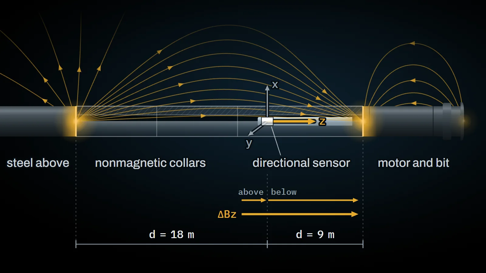
Steel above and below the tool can produce predominantly axial interference. That component mainly affects the axial magnetometer. Cross-axial interference can also occur, so the two cross-axial sensors are not protected from every magnetic disturbance. Sufficient nonmagnetic drill collar (NMDC) spacing reduces the influence of nearby magnetic components.
 (opens the full-size image)
ModelPole model after Grindrod and Wolff (1983), with 200 µWb poles; diameters are exaggerated.
The short collar calculation uses the accelerometers, the two cross-axial magnetometers, and reference field strength and dip information. It substitutes for the excluded axial measurement. The equations and numerical solution depend on the implementation.
The approach appears in Russell and Russell's 1979 patent. Russell and Roesler described its commercial application in SPE/IADC 13476 in 1985. Full-scale laboratory tests in simulated horizontal wells later reported azimuth-error reductions of up to a factor of ten in east-west wells (Cheatham et al., SPE 23852). Those results describe the tested tools, interference, and reference conditions. They do not establish performance for every field application.
Planning magnetic isolation
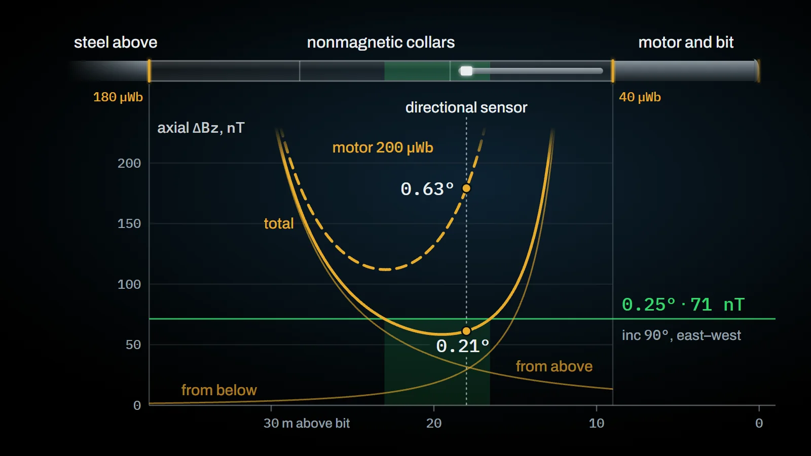
NMDC spacing depends on the BHA's magnetic pole strengths, the sensor position, the planned well attitude, and the local magnetic field. Grindrod and Wolff's 1983 spacing method used field measurements to support these calculations.
Chapter 5.2 of An Introduction to Wellbore Positioning includes an example based on a possible azimuth error of 0.25°. Using 18.9 m of NMDC where the calculation required 24 m increases the estimated possible error to about 0.4°, under the example's inverse-square spacing relationship.
The book warns against reducing NMDC and then correcting the survey with that spacing formula. Its assumed pole strengths may not represent the actual BHA. This warning concerns that theoretical correction; it does not establish a general ban on planning a validated magnetic correction service.
Magnetisation can also change during a run. Magnetic particle inspection can leave remanent magnetisation, and mechanical strain can change it. Nominally nonmagnetic components can have local magnetic imperfections. BHA magnetisation studies and correction methods describe these effects. Adequate planned spacing therefore requires confirmation from the acquired data.
 (opens the full-size image)
ModelPole model after Grindrod and Wolff (1983); horizontal east–west well, 56,000 nT field, 73° dip. Green marks the sensor positions that meet 0.25°.
Geometry and correction limits
For a small, purely axial field error, the first-order magnitude of the conventional azimuth error is approximately:
|ΔAz| ≈ |ΔBz · sin(inc) · sin(az)| / |B · cos(dip)|
Here, ΔAz is in radians. ΔBz is the axial field error, and B is the undisturbed total field strength. Both use the same field units. The approximation assumes a nonzero horizontal field and a defined azimuth. Inclination inc is measured from vertical, az is azimuth from magnetic north, and dip is the magnetic dip angle. B·cos(dip) is the horizontal magnetic field. The absolute values show the magnitude without prescribing a sensor-axis sign convention. This is the geometry used by the ISCWSA axial interference weighting function.
- Horizontal magnetic east-west wells have the greatest sensitivity to a small axial interference component.
- Magnetic north-south wells have zero first-order azimuth sensitivity to that component. Field strength and dip can still change.
- A weaker horizontal magnetic field increases sensitivity. This often makes axial interference more significant at high magnetic latitudes.
In the ideal short collar calculation, excluding the axial measurement removes its direct interference contribution. The result still depends on the cross-axial measurements, the accelerometers, and the magnetic reference. Their errors remain relevant.
The corrected azimuth weighting functions contain the denominator 1 − sin²(inc)·sin²(az). It approaches zero near horizontal magnetic east-west, making the calculation sensitive to small input errors. A controlled laboratory improvement does not remove this reference and sensor uncertainty.
Chapter 13.1 of the Wellbore Positioning e-book recommends avoiding the described axial correction above 70° inclination within 20° of magnetic east or west. For an actual operation, use the limits of the validated tool and correction procedure.
The gravity, field-strength, and dip checks also have geometric limits. Axial interference can produce field-strength and dip residuals whose sizes and signs depend on inclination, azimuth, and magnetic dip. At horizontal magnetic east-west, both magnetic checks lose first-order sensitivity to a purely axial disturbance. Passing them cannot independently confirm the azimuth.
Matching the error model to the calculation
The standard model includes axial magnetometer uncertainty and the drillstring interference term AMIL. The generic AMIL magnitude is 220 nT at 1σ. Its azimuth weighting follows the first-order relationship above.
For example, a total field of 56,000 nT and a dip of 73° give a horizontal field of about 16,400 nT. In a horizontal magnetic east-west well, 220 nT corresponds to approximately 0.77° of azimuth uncertainty at 1σ. Its share of the total position uncertainty depends on the complete tool model and trajectory.
The axial-corrected model, commonly identified by +AX and historically by MWD+SC, excludes the axial magnetometer terms and AMIL. It uses the corrected sensor weighting functions and includes MFI and MDI: uncertainty in the reference total field and dip.
Those reference inputs affect the short collar azimuth calculation. They also support QC, but do not enter the conventional six-axis magnetic azimuth calculation directly. Declination uncertainty affects both methods when the magnetic azimuth is converted to true or grid north.
The following values are historical examples from Maus and Croke's 2014 presentation, rather than current accuracy guarantees:
| Reference in the 2014 study | Total field uncertainty, 1σ | Dip uncertainty, 1σ |
|---|---|---|
| IGRF / WMM | 157 nT | 0.24° |
| BGGM, 2014 example | 130 nT | 0.20° |
| HDGM | 107 nT | 0.16° |
| IFR1 | 50 nT | 0.10° |
| IFR2, study assumption | 40 nT | 0.08° |
The presentation, slide 7 explicitly identifies the IFR2 values as assumptions used in that study. The BGGM category also changed after 2019 in the ISCWSA reference classification. Use uncertainty values that match the selected reference, version, and validated performance.
Rev5 divides the reference families into omission, commission, and other components. These support the treatment of correlation between wells, as explained in the main field model article.
The ISCWSA generic tool codes are conservative defaults for cases without a tool-specific model. Selection must account for the actual azimuth calculation, reference, and corrections. A planned long collar survey delivered using the five-axis correction requires a model for that delivered method.
MSA is a separate processing choice. It can estimate and correct an axial bias across several stations without replacing the six-axis calculation with a single-station five-axis calculation. Use the model appropriate to the validated MSA process. The published correction-model examples distinguish MSA and axial correction variants.
A 1σ magnitude is not an acceptance bound for an individual run. The model includes systematic errors that can persist across its stations. A persistent error does not, by itself, invalidate a population's zero-mean assumption. Investigate a demonstrated bias, correct a significant supported bias, and assess the residual uncertainty.
For scale, Maus and DeVerse's Eagle Ford case reported 445 nT of axial interference and an average azimuth correction of about 0.65°. They estimated a lateral displacement of approximately 113 ft for a 10,000 ft lateral with that angular error. Those values depend on that case's field and well direction.
Checking the survey data
Field acceptance criteria (FAC) compare measured gravity, field strength, and dip with their references. Model-derived QC limits account for the selected tool model, station attitude, location, and reference uncertainty. The operator's procedure specifies the acceptance criterion and response to a failed check.
Maus and Croke reported the following global average 1σ errors in 2014. These are neither station-specific values nor operational acceptance limits:
| Model in the 2014 study | Field-strength error, 1σ | Dip error, 1σ |
|---|---|---|
| MWD, standard | 217 nT | 0.33° |
| MWD+AX | 103 nT | 0.15° |
| MWD+IFR1 | 180 nT | 0.28° |
| MWD+IFR1+AX | 66 nT | 0.09° |
Source: Maus and Croke, slide 23. Their presentation proposed a screening criterion of no more than 10% of stations failing the chosen 2σ QC criteria. It was a suggestion, rather than a universal ISCWSA acceptance rule.
Retain the raw measurements and their residuals, as well as the corrected data. A correction can reduce disagreement with the same reference used to calculate it. That agreement alone is not an independent accuracy check.
FAC also cannot detect every survey error. For example, tool-to-borehole misalignment and sag can affect the trajectory without producing a corresponding failure in these scalar checks. The FAC study identifies this limitation.
Trends across stations can support an interference diagnosis. They do not automatically establish its cause or justify a correction.
Checking the magnetic reference
A residual is the measured value minus its reference. It can reflect reference error, axial or cross-axial interference, calibration error, or noise. A single-station correction cannot separate all these causes.
In Maus and DeVerse's published Bakken and Eagle Ford examples, differences between global-model and IFR declination estimates were typically around 0.5° and exceeded 1° in some areas. Their field-strength example showed a raw-survey misfit near 500 nT against IGRF and about 375 nT against the IFR reference. This compares two reference estimates; it does not establish an error-free measurement of the local field.
Using an unsuitable reference in a correction can have three consequences:
- Corrected field strength and dip can move closer to that reference. This can make the residuals misleading as an accuracy check.
- Reference error can enter the corrected azimuth, with sensitivity increasing near horizontal magnetic east-west.
- An unsuitable reference uncertainty can make the reported position uncertainty too small. The +AX calculation does not guarantee a smaller ellipse, particularly near its geometric limits.
A reference mismatch can also cause otherwise usable data to fail FAC. Check the reference and the measurements before changing or rejecting the survey.
Selecting and validating a correction
Five checks help assess whether a correction is supported:
-
Validate the reference. Check coordinates, depth, date, model version, and any local or time-dependent corrections. IFR1 addresses local crustal contributions; IFR2 also addresses time-dependent disturbance fields. Update frequency alone does not establish reference quality. A better reference reduces one uncertainty source; remaining residuals can still have several causes.
-
Assess the available variation. Changes in inclination, azimuth, and toolface help separate error parameters. A tangent section can support some estimates, while leaving others strongly correlated. Check which parameters the data can resolve, rather than assuming that every parameter is identifiable.
-
Check the MSA assumptions and uncertainty. MSA estimates common sensor errors across several stations. Nyrnes et al., SPE/IADC 125677 describe minimum requirements; the ISCWSA discussion includes tangent and changing-attitude sections. Bulychenkov's 2013 study described a limitation near 55° inclination for an east-west, BGGM-based approach. It also described a modified method that could overcome that limitation with sufficient trajectory variation. That number is not a universal limit for every MSA implementation.
-
Compare runs and nearby wells. Consider the BHA, tool, acquisition times, locations, and reference methods. Interference can change during a run; reference errors can vary with location and time. Repeated patterns provide diagnostic evidence, rather than proof of one cause. Residuals near existing casing can indicate external interference. A standard axial correction does not address arbitrary external magnetic interference.
-
Use an independent survey where needed. A suitable gyro survey can test magnetic azimuths without using the local magnetic field. Its initialization must not depend on the disputed magnetic azimuth. Compare the surveys in the same reference frame and account for both uncertainties, including tool alignment and depth matching.
The resulting wellsite checklist is:
- Plan suitable magnetic isolation for the BHA and survey requirements.
- Validate the magnetic reference and retain raw station data.
- Assess residual trends and the parameters the available geometry can resolve.
- Apply supported corrections within the validated procedure's limits.
- Use independent checks where the remaining ambiguity affects the decision.
- Report the delivered calculation, reference, corrections, model, and residual uncertainty.
References
- Russell, M.K. and Russell, A.W. (1979). Surveying of Boreholes. US Patent 4,163,324.
- Grindrod, S.J. and Wolff, J.M. (1983). Calculation of NMDC Length Required for Various Latitudes Developed From Field Measurements of Drill String Magnetisation. IADC/SPE 11382.
- Russell, A.W. and Roesler, R.F. (1985). Reduction of Nonmagnetic Drill Collar Length Through Magnetic Azimuth Correction Technique. SPE/IADC 13476.
- Cheatham, C.A. et al. (1992). Effects of Magnetic Interference on Directional Surveys in Horizontal Wells. IADC/SPE 23852.
- Brooks, A.G., Gurden, P.A., Noy, K.A. (1998). Practical Application of a Multiple-Survey Magnetic Correction Algorithm. SPE 49060.
- Williamson, H.S. (2000). Accuracy Prediction for Directional Measurement While Drilling. SPE Drilling & Completion 15(4), SPE 67616.
- Ekseth, R. et al. (2006). The Reliability Problem Related to Directional Survey Data. IADC/SPE 103734.
- Nyrnes, E., Torkildsen, T., Wilson, H. (2009). Minimum Requirements for Multi-Station Analysis of MWD Magnetic Directional Surveys. SPE/IADC 125677.
- Brooks, A.G. (2012). Multi-Station Analysis of Magnetic Surveys. US Patent 8,280,638.
- Bulychenkov, K. (2013). Improving Multistation Analysis of MWD Directional Magnetic Surveys. SPE 166865.
- Maus, S. and Croke, R. (2014). Field Acceptance Criteria Based on ISCWSA Tool Error Models. ISCWSA Meeting 39, slides 7 and 23–25.
- Maus, S. and DeVerse, S. (2015). Enhanced Wellbore Placement Accuracy Using Geomagnetic In-Field Referencing and Multi-Station Correction. URTeC 2173526.
- Grindrod, S.J. et al. (2016). OWSG Standard Survey Tool Error Model Set for Improved Quality and Implementation in Directional Survey Management. IADC/SPE 178843.
- ISCWSA. Definition of the ISCWSA Error Model, Rev 5.13, sections 4.7, 6.2, 6.3.7, and 7.
- ISCWSA. Five Primary Geomagnetic Reference Model Categories.
- Jamieson, A. et al. An Introduction to Wellbore Positioning, version V09.10.17, chapters 5.2 and 13.1.